Evaluating the Moneyball draft eleven years later:Part 2: Value of the major leaguers, college vs. high school draftees

If you read the book or saw the movie Moneyball, a strong impression you could come away with is that Billy Beane had helped make the Oakland A's a better team than their payroll predicted they should be by using modern approaches for scouting talent. The book pays a lot of attention to the 2002 baseball draft, a draft where Beane chose only college players and left out the high school stars. The emotional reason behind this decision is that Beane himself had been drafted out of high school and did not turn out to be productive at the major league level.

Obviously, a sample size of n = 1 is not a basis for science. Let's look at a statistic from the high school and college players among the first 50 drafted position players and the first 50 drafted pitched.

I admit that a single statistic measures only a single dimension and baseball is not a one dimensional game. For position players, I'm using total bases, which means adding up the hits and walks and stolen bases, giving one extra base for each double, two extra bases for each triple, three extra for a home run and subtracting the number of times the player was caught stealing.

For the pitchers, I use innings pitched as the measure of their value over their career. It's not perfect, as it tends to favor starting pitchers over relievers, but in general it does show over a career how much value a pitcher had for his club.

Total base numbers for the players from the 2002 draft that made the majors
High school draftees 
===============
2902, 2114, 2111, 2062, 1629, 1243, 907, 527, 476, 179, 98, 54, 19
Average: 1101.6
Standard deviation: 846.5
n = 13

College draftees
===========
2670, 2649, 1928, 1292, 1270, 1100, 829, 541, 424, 124, 6, 3, 2
Average: 987.5
Standard deviation: 951.0
n = 13

For these numbers, the high schoolers are better prospects on average than the college players, due in large part to the most productive hitter on the list, Prince Fielder and his 2,902 career total bases so far. The top two college recruits were Nick Swisher and Curtis Granderson, who are also both still active.

The reason I included the standard deviation and the sample size is to find out if the difference we see is statistically significant and the answer is no. The simplest formula for statistical significance is the z-score method, and the big standard deviations are in the denominator of the formula, which overwhelm the numerator by a lot.

Innings pitched numbers for the players from the 2002 draft that made the majors
High school draftees 
===============
1537, 1492, 1377, 1163, 1022, 473, 450, 233,180, 164, 120, 15, 10
Average = 633.5
Standard deviation = 529.3
n = 13

College draftees
===========
1438, 1202, 1179, 1161, 1141, 495, 166, 157, 114, 82, 68, 20
Average = 602
Standard deviation = 491.2
n = 12

Once again, the big standard deviations mean the difference isn't significant, but the high school draftees did slightly outshine the college.

Generally, Beane's decision to ignore high school talent appears to be counter-productive. On average, they are no more likely to wash out than college players and the most talented can be in the major leagues at a younger age with a chance to have a longer career if they can stay healthy and productive.

One of the reasons the book focused on the draft was that the Athletics had negotiated a large number of first round picks in 2002, the highest being the 16th overall and the lowest being the 39th. Tomorrow, we will look at those picks and how the A's did against their competitors.

Evaluating the Moneyball draft eleven years later.Part 1: Making the majors or not

Michael Lewis' book Moneyball concentrated on the Oakland A's in 2002, more on the front office than on the players on the field. The idea was that general manager Billy Beane and his employees were looking at new and better ways to develop talent and use it, giving them a chance to be competitive with teams whose payrolls were several times higher than what the frugal A's ownership was willing to spend.

Beane and his team used sabremetrics, a word coined from the acronym SABR, the Society of American Baseball Research. The idea was that he would be able to draft players under-appreciated by other clubs and build a nucleus of young talent, though the best would be lost to free agency within a few years.

Beane's method really wasn't that scientific. What Billy Beane wanted to avoid was drafting another Billy Beane. He was much sought after out of high school. He debated whether he would go to college or go straight into baseball out of high school. He was drafted out of high school and he made the major leagues eventually, but he wasn't the All-Star the scouts had hoped he would be.

Beane the general manager drafted no high school players in 2002, worried there was a high probability he might find too many kids like himself who crumbled under the pressure of professional baseball.

Using the 2002 draft as our data set, let's ask the question: Is there a significant difference between the success rates of high school and college draftees?

The null hypothesis: There is no significant difference.
Data set #1: The first 50 position players drafted
Data set #2: The first 50 pitchers drafted
How we split the sets: A player was either drafted from high school or college and the player either made the major league roster or did not.
We will perform a chi-square test to see if the differences we see are significant.

Problem with this test: We are lumping together some players with very good careers so far with some guys who just barely had a cup of coffee in The Show. That problem will be addressed in the test used tomorrow.

Position players
============
High school draft: 13 made the majors, 13 did not
College draft: 13 made the majors, 11 did not

Test statistic: chi square = 0.087, well below even the 90% confidence threshold of 2.706


Pitchers
======
High school draft: 13 made the majors, 10 did not
College draft: 12 made the majors, 15 did not

Test statistic: chi square = 0.725, well below even the 90% confidence threshold of 2.706

These numbers just count whether players will make it to the majors or not, and as we can see, out of the first hundred or so players chosen, about half will see major league experience and high school draftees are not significantly different from college draftees. Another question is how good are those major leaguers when we compare the high schoolers to the collegiates?  Tomorrow, we will use a different statistical test on only one stat per player, not a completely fair test, but it does give an approximate idea of the players' worth to their squads.

The Statistical World: Part 2

As someone who use to gamble much more than I do now,  I have a visceral understanding of probability that non-gamblers do not have.

For example, if we reach this position in a game of backgammon, here are the odds of winning.

If it's black's turn: game over. Black wins 100% of the time.

If it's White's turn: There are exactly 19 rolls that win and 17 rolls that lose. It's a little better than flipping a fair coin, which would be 50%-50%. This rounds to 52.8% chance to win and a 47.2% chance to lose.

The only thing to question is if "fair dice" exist, or even "fair coins". Lots of data has been compiled and the answer is yes. Most coins in your pocket will come up heads when flipped about 50% of the time, and most dice have a roughly even distribution of the six possible numbers.

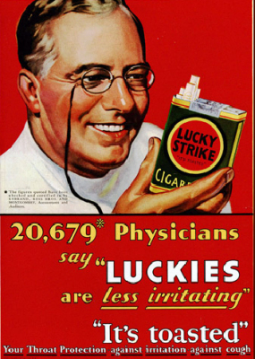
And then there is randomness in the real world. if you saw the first episode of Mad Men, you might recall that the Surgeon General's 1960 report on the effects of smoking and the subsequent publishing in Reader's Digest was a major plot point. To drive home the point that Don Draper is not just a pretty face, he comes up with the Lucky Strike slogan "It's toasted" on the spot when pitching to the worried owners.

If fact, the slogan is real and pre-dates the 1960 advertising crisis by several years. Mad Men's first episode gets several things right, including that the tobacco industry would be barred from using testimonials from doctors or even dentists in the years to come.

But what are the exact probabilities of cigarette smoking causing you harm and shortening your life? Here the numbers get hazy. Many different factors can be considered other than smoking, some that make things better and some that make things worse. It is about as far as you can get from an exact science, but serious experts take randomness into account and still claim smoking has multiple ways it can screw up your health, many of them very significant changes for the worse indeed.

Tomorrow, we talk about the randomness.